We’re captive on the carousel of time
We can’t return we can only look behind
From where we came
And go round and round and round
In the circle game
– Joni Mitchell, The Circle Game
All living things change over time, and this evolution can be quantitatively measured and analyzed. Mathematics makes use of equations to define models that change with time, known as dynamical systems. In this unit we will learn how to construct models that describe the time-dependent behavior of some measurable quantity in life sciences. Numerous fields of biology use such models, and in particular we will consider changes in population size, the progress of biochemical reactions, the spread of infectious disease, and the spikes of membrane potentials in neurons, as some of the main examples of biological dynamical systems.
Many processes in living things happen regularly, repeating with a fairly constant time period. One common example is the reproductive cycle in species that reproduce periodically, whether once a year, or once an hour, like certain bacteria that divide at a relatively constant rate under favorable conditions. Other periodic phenomena include circadian (daily) cycles in physiology, contractions of the heart muscle, and waves of neural activity. For these processes, theoretical biologists use models with discrete time, in which the time variable is restricted to the integers. For instance, it is natural to count the generations in whole numbers when modeling population growth.
This chapter will be devoted to analyzing dynamical systems in which time is measured in discrete steps. In this chapter you will learn to do the following:
write down discrete-time (difference) equations based on stated assumptions
find analytic solutions of linear difference equations
use for loops in R
compute numeric solutions of difference equations
8.1 Discrete time population models
Let us construct our first models of biological systems. We will start by considering a population of some species, with the goal of tracking its growth or decay over time. The variable of interest is the number of individuals in the population, which we will call \(N\). This is called the dependent variable, since its value changes depending on time; it would make no sense to say that time changes depending on the population size. Throughout the study of dynamical systems, we will denote the independent variable of time by \(t\). To denote the population size at time \(t\), we can write \(N(t)\) but sometimes use \(N_t\).
8.1.1 static population
In order to describe the dynamics, we need to write down a rule for how the population changes. Consider the simplest case, in which the population stays the same for all time. (Maybe it is a pile of rocks?) Then the following equation describes this situation: \[N(t+1) = N(t) \] This equation mandates that the population at the next time step be the same as at the present time \(t\). This type of equation is generally called a difference equation, because it can be written as a difference between the values at the two different times: \[N(t+1) - N(t) = 0\] This version of the model illustrates that a difference equation at its core describes the increments of \(N\) from one time step to the next. In this case, the increments are always 0, which makes it plain that the population does not change from one time step to the next.
8.1.2 exponential population growth
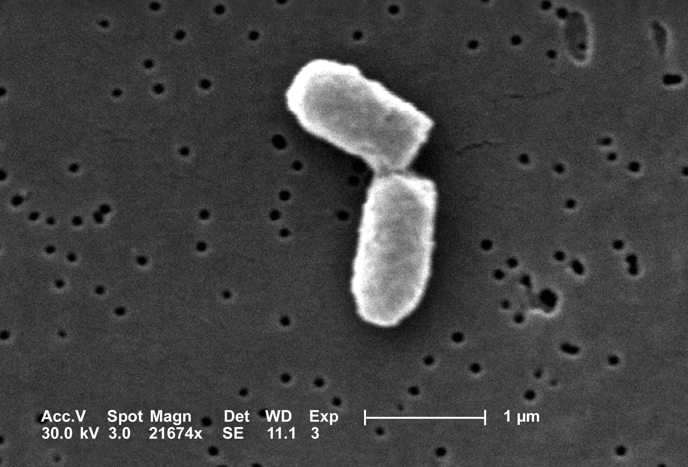
Let us consider a more interesting situation: as a colony of dividing bacteria, such as E. coli, shown in figure \(\ref{fig:ch14_cell_div}\). We will assume that each bacterial cell divides and produces two daughter cells at fixed intervals of time, and let us further suppose that bacteria never die. Essentially, we are assuming a population of immortal bacteria with clocks. This means that after each cell division the population size doubles. As before, we denote the number of cells in each generation by \(N(t)\), and obtain the equation describing each successive generation: \[ N(t+1) = 2N(t)\] It can also be written in the difference form, as above: \[ N(t+1) - N(t) = N(t) \] The increment in population size is determined by the current population size, so the population in this model is forever growing. This type of behavior is termed exponential growth, which we will investigate further in section \(\ref{sec:math14}\).
Scanning electron micrograph of a dividing Escherichia coli bacteria; image by Evangeline Sowers, Janice Haney Carr (CDC) in public domain via Wikimedia Commons.
8.1.3 population with births and deaths
Suppose that a type of fish lives to reproduce only once after a period of maturation, after which the adults die. In this simple scenario, half of the population is female, a female always lays 1000 eggs, and of those, 1% survive to maturity and reproduce. Let us set up the model for the population growth of this idealized fish population. The general idea, as before, is to relate the population size at the next time step \(N(t+1)\) to the population at the present time \(N(t)\).
Let us tabulate both the increases and the decreases in the population size. We have \(N(t)\) fish at the present time, but we know they all die after reproducing, so there is a decrease of \(N(t)\) in the population. Since half of the population is female, the number of new offspring produced by \(N(t)\) fish is \(500N(t)\). Of those, only 1% survive to maturity (the next time step), and the other 99% (\(495N(t)\)) die. We can add all the terms together to obtain the following difference equation: \[
N(t+1) = N(t) - N(t) + 500N(t) - 495 N(t) = 5N(t)
\]
The number 500 in the expression is the birth rate of the population per individual, and the negative terms add up to the death rate of 496 per individual. We can re-write the equation in difference form: \[
N(t+1) - N(t) = 4N(t)
\]
This expression again generates growth in the population, because the birth rate outweighs the death rate.
8.1.4 dimensions of birth and death rates
As we discussed in section \(\ref{sec:model2}\) the dimensions of quantities in a model have to satisfy the rules of dimensional analysis we discussed in chapter 2. In the case of population models, the birth and death rates measure the number of individuals that are born (or die) within a reproductive cycle for every individual at the present time. Their dimensions must be such that the terms in the equation all match: \[ [N(t+1) - N(t)] = [population] = [r] [N(t)] = [r] \times [population] \] This implies that \(r\) is algebraically dimensionless. However, the meaning of \(r\) is the rate of change of population over one (generation) time step. \(r\) is the birth or death rate of the population per generation, and therefore, when such rates are measured, they are reported with units of inverse time (e.g. number of offspring per year).
8.1.5 linear demographic models
We will now write a general difference equation for any population with constant birth and death rates. This will allow us to substitute arbitrary values of the birth and death rates to model different biological situations. Suppose that a population has the birth rate of \(b\) per individual, and the death rate \(d\) per individual. Then the general model of the population size is: \[\begin{equation}
N(t+1) = (1 + b - d)N(t)
\label{linear_pop}
\end{equation}\]
The general equation also allows us to check the dimensions of birth and death rates, especially as written in the incremental form: \(N(t+1) - N(t) = (b - d)N(t)\). The change in population rate over one reproductive cycle is given by the current population size multiplied by the difference of birth and death rates, which as we saw are algebraically dimensionless. The right hand side of the equation has the dimensions of population size, matching the difference on the left hand side.
8.2 Solutions of linear difference models
8.2.1 simple linear models
Having set up the difference equation models, we would naturally like to solve them to find out how the dependent variable, such as population size, varies over time. A solution may be analytic, meaning that it can be written as a formula, or numeric, in which case it is generated by a computer in the form of a sequence of values of the dependent variable over a period of time. In this section, we will find some simple analytic solutions and learn to analyze the behavior of difference equations which we cannot solve exactly.
NoteDefinition
A function \(N(t)\) is a solution of a difference equation \(N(t+1) = f(N(t))\) if it satisfies that equation, i.e. when \(N(t)\) is plugged into both sides, they match exactly.
For instance, let us take our first model of the static population, \(N(t+1) = N(t)\). Any constant function is a solution, for example, \(N(t) = 0\), or \(N(t) = 10\). There are actually as many solutions as there are numbers, that is, infinitely many! In order to specify exactly what happens in the model, we need to specify the size of the population at some point, usually, at the “beginning of time”, \(t = 0\). This is called the initial condition for the model, and for a well-behaved difference equation it is enough to determine a unique solution. For the static model, specifying the initial condition is the same as specifying the population size for all time.
Now let us look at the general model of population growth with constant birth and death rates. We saw in equation \(\ref{linear_pop}\) above that these can be written in the form \(N(t+1) = (1 + b - d) N(t)\). To simplify, let us combine the numbers into one growth parameter \(r = 1 + b - d\), and write down the general equation for population growth with constant growth rate: \[N(t+1) = rN(t)\]
To find the solution, consider a specific example, where we start with the initial population size \(N_0 = 1\), and the growth rate \(r=2\). The sequence of population sizes is: 1, 2, 4, 8, 16, etc. This is described by the formula \(N(t) = 2^t\).
In the general case, each time step the solution is multiplied by \(r\), so the solution has the same exponential form. The initial condition \(N_0\) is a multiplicative constant in the solution, and one can verify that when \(t=0\), the solution matches the initial value:
I would like the reader to pause and consider this remarkable formula. No matter what the birth and death parameters are selected, this solution predicts the population size at any point in time \(t\).
In order to verify that the formula for \(N(t)\) is actually a solution in the meaning of definition \(\ref{def:math14_sol}\), we need to check that it actually satisfies the difference equation for all \(t\), not just a few time steps. This can be done algebraically by plugging in \(N(t+1)\) into the left side of the dynamic model and \(N(t)\) into the right side and checking whether they match. For \(N(t)\) given by equation \(\ref{eq:lin_discrete_sol}\), \(N(t+1) = r^{t+1} N_0\), and thus the dynamic model becomes: \[r^{t+1} N_0 = r \times r^t N_0\]
Since the two sides match, this means the solution is correct.
8.2.2 models with a constant term
Now let us consider a dynamic model that combines two different rates: a proportional rate (\(rN\)) and a constant rate which does not depend on the value of the variable \(N\). We can write such a generic model as follows: \[ N(t+1) = rN(t) + a \]
The right-hand side of this equation is a linear function of \(N\), so this is a linear difference equation with a constant term. What function \(N(t)\) satisfies it? One can quickly check that that the same solution \(N(t) = r^t N_0\) does not work because of the pesky constant term \(a\): \[ r^{t+1} N_0 \neq r \times r^t N_0 + a\]
To solve it, we need to try a different form: specifically, an exponential with an added constant. The exponential can be reasonably surmised to have base \(r\) as before, and then leave the two constants as unknown: \(N(t) = c_1 r^t + c_2\). To figure out whether this is a solution, plug it into the linear difference equation above and check whether a choice of constants can make the two sides agree: \[ N(t+1) = c_1 r^{t +1} + c_2 = rN(t) + a = rc_1 r^t + rc_2+ a\] This equation has the same term \(c_1 r^{t +1}\) on both sides, so they can be subtracted out. The remaining equation involves only \(c_2\), and its solution is \(c_2 = a/(1-r)\). Therefore, the general solution of this linear difference equation is the following expression, which is determined from the initial value by plugging \(t=0\) and solving for \(c\).
\[\begin{equation}
N(t) = c r^t + \frac{a}{1-r}
\label{eq:ch14_sol_wconst}
\end{equation}\]
Example. Take the difference equation \(N(t+1) = 0.5 N(t) + 40\) with initial value \(N(0)= 100\). The solution, according to our formula is \(N(t) = c 0.5^t + 80\). At \(N(0) = 100 = c+80\), so \(c=20\). Then the compete solution is \(N(t) = 20 \times 0.5^t + 80\). To check that this actually works, plug this solution back into the difference equation: \[ N(t+1) = 20 \times 0.5^{t+1} + 80 = 0.5 \times (20 \times 0.5^t + 80) + 40 = 20 \times 0.5^{t+1} + 80\] The equation is satisfied and therefore the solution is correct.
8.2.3 population growth and decline
The parameter \(r\) can assume different values, depending on the birth and death rates. If the birth rate is greater than the death rate, \(r > 1\), and if it is the other way around, \(r < 1\). Note that for a realistic biological population, the death rate is limited by the number of individuals present in the population. The maximum number of individuals at any time is \(N(t)+bN(t)\), so this means that \(d \leq b +1\). Therefore, for a biological population, \(r \geq 0\).
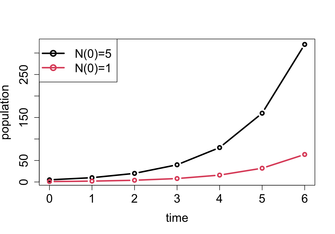
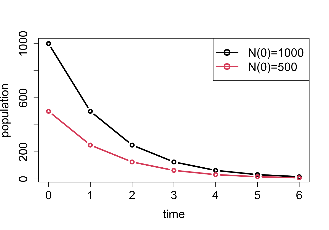
Plots of solutions of linear difference equations: a) \(N(t+1) = 2N(t)\) with different initial values; b) \(N(t+1) = 0.5N(t)\) with different initial values
Plots of solutions of linear difference equations: a) \(N(t+1) = 2N(t)\) with different initial values; b) \(N(t+1) = 0.5N(t)\) with different initial values
The solutions in formula \(\ref{eq:lin_discrete_sol}\) and \(\ref{eq:ch14_sol_wconst}\) are exponential functions, which as we saw in section \(\ref{sec:math2}\) have a limited menu of behaviors, depending on the value of \(r\). If \(r > 1\), multiplication by \(r\) increases the size of the population, so the solution \(N(t)\) will grow. If \(r < 1\), multiplication by \(r\) decreases the size of the population, so the solution \(N(t)\) will decay (see figure \(\ref{fig:ch14_solutions}\)). Finally, if \(r=1\), multiplication by \(r\) leaves the population size unchanged, like in the pile of rocks model. Here is the complete classification of the behavior of population models with constant birth and death rates (assuming \(r>0\)):
\(r > 1\): \(N(t)\) grows without bound
\(r < 1\): \(N(t)\) decays to the constant \(a/(1-r)\)
\(r = 1\): \(N(t)\) remains constant
As we see, there are only two options for solution of linear difference equations: ever-faster growth or decay to zero or another constant value. The exponential growth of populations is also known as after the early population modeler Thomas Malthus. He used a simple population model with constant growth rate to predict demographic disaster due to the exponentially increasing population outstripping the growth in food production. In fact, human population has not been growing with a constant birth rate, and food production has (so far) kept up pace with population size, illustrating yet again that mathematical models are only as good as the assumptions that underlie them.
8.2.4 Exercises
For the following scenarios for a population:
Build a dynamic model by writing down a difference equation in the updating function form (with the value of the variable at time step \(t+1\) on the left hand side and the value of the variable at time step \(t\) on the right);
find the solution of the linear difference equation with a generic/unknown initial value and verify that it satisfies the difference equation by plugging the solution into your model;
use the given initial value to predict the value at a future time step.
8.2.4.1 Model scenarios
Suppose the number of trees in a planted forest decreases by 50 every year (as they are harvested) and no new trees are planted. If there are 3000 trees initially, how many will be be after 10 years?
Zombies have appeared in Chicago. Every day, each zombie produces 3 new zombies and none are killed. If there is one zombie initially, how many zombies will there be in 7 days?
Suppose hunters kill 50 deer in a national forest every hunting season, while the deer by themselves have equal birth and death rates. If there are initially 500 deer in the forest, predict how many there will be in 5 years.
The concentration of a drug in the bloodstream decreases by 20% every hour. If the initial concentration is 400 (arbitrary units), what is the concentration after 24 hours?
The number of infected people in a population grows by 8% per day and those who become infected remain infected. If initially there are 8 infected, how many will be infected in 45 days?
Suppose bacteria in a population divide in 2 every hour and 90% of the current population dies after reproduction, not including the new offspring. If the population initially has 10 million bacteria, predict how many there will be in 12 hours.
In a rabbit population, each pair produces 1.2 offspring every year (i.e. 0.6 per capita, assuming the whole population is paired up into mating pairs) and the adults have a 0.5 annual death rate after reproduction. If initially there are 100 rabbits, predict how many there will be in 5 years.
Consider a rabbit population with the same birth and death rates as in question 7, but now a python that lives nearby eats exactly 1 rabbit per month. If initially there are 100 rabbits, how many do you predict will be in 10 years?
10 fish are added to an aquarium every month, while 80% of those present survive every month and there is no reproduction. If initially there are 10 fish in the aquarium, predict how many there will be in 2 years.
A gene has length of 10000 nucleotides, some of them are ancestral (A) and others are mutant letters (M). Every generation 2% of the ancestral letters become mutant and 1% of the mutant letters revert to the ancestral state. Write a discrete time model for the number of the mutant nucleotides M (Hint: \(A = 10000 - M\)). If initially there are 0 mutant letters (all 10000 are ancestral), predict how many there will be in 10 generations.
Twenty flies fly into a house every day, and half of the flies in the house at beginning of each day find their way out (no births or deaths happen in the house.) If there are 10 files in the house initially, how many will there be in 12 days?
Suppose that a branch grows at the rate of 10 cm a month (year round, assume no seasonal variations) and every month a gardener trims 25% of the length of the branch. If initially the branch is 10 cm long, what will be its length in 6 months?